| Loading ITables v2.8.0 from the internet... (need help?) |
You don't need error nodes, you need better features
mechinterp
This post is a follow-up to the methods I developed in the previous post on replacement-aware training.
1 Summary
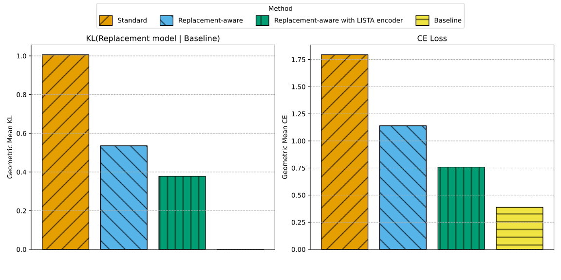
A replacement model (Ameisen et al. 2025) is a modification to an LLM in which some subset of internal activations are replaced with ones computed as a sum of more interpretable features, such as those found by sparse auto-encoders (SAEs) (Cunningham et al. 2023) or cross-layer transcoders (CLTs) (Lindsey et al. 2024). When multiple components are thus re-encoded, methods inspired by structural equation modeling can be applied to construct feature circuits (Marks et al. 2024) that attempt to explain some aspect of the model’s behavior in terms of these features. Because the re-encoding process is inherently lossy, errors from earlier components compound in later ones, resulting in severely damaged performance. In fact, applying current SAEs to just a few layers generally results in a replacement model that is no longer recognizable as a language model; it is unable to generate coherent output at all. To mitigate this effect, Marks et al. (2024) introduce error nodes into their recovered causal model, with values set such that they exactly cancel the re-encoding error of the corresponding SAE. I find this approach deeply unsatisfying, as I outline in Section 2.2.
In this post, I present an alternative to error nodes: train SAEs that are robust to upstream errors. I call this approach replacement-aware training because it involves introducing a loss term for each SAE that penalizes distortions to the next layer’s features, more closely matching the replacement model use case. I previously applied this method to a toy language model, and have now scaled it up to Gemma-2-2B (Gemma Team et al. 2024). The result is a suite of residual stream SAEs that can be used as-is in a full replacement model, which despite degraded performance, still retains language capabilities. I have made the code and weights for these SAEs publicly available; instructions for downloading and running them are available here.
I consider the methods outlined in this post an existence proof of the claim asserted in the title; they are by no means optimal. My overall approach was to keep adding to a bag of stackable tricks such that I could attain the goal of running a replacement model with mostly retained capabilities. While it does appear that no one innovation is sufficient on its own, I suspect that simplifications can be made, which I leave to future work. My core findings are:
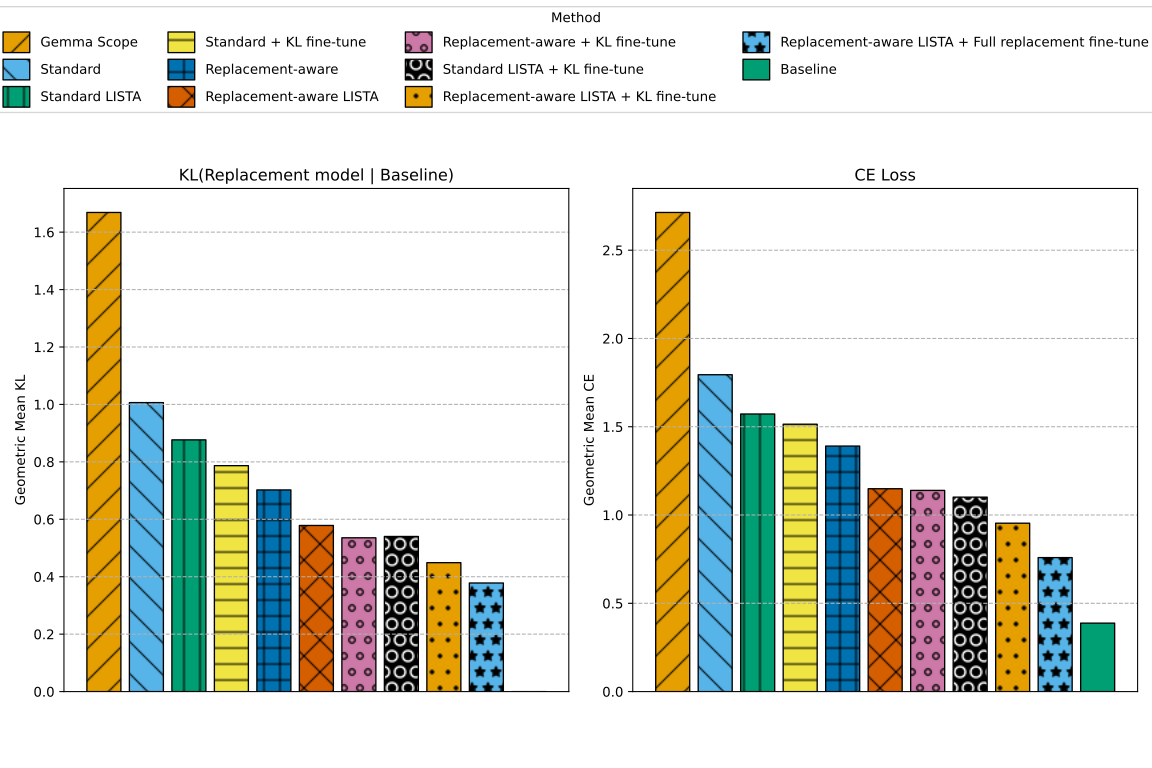
- Replacement-aware training greatly reduces KL divergence between the replacement model and base model as compared to standard methods, without sacrificing faithfulness;
- A short (~1 million tokens) encoder-only fine-tuning stage can further reduce KL divergence, and this is effective even on replacement-naive SAEs;
- Using a more powerful encoder based on LISTA (Gregor and LeCun 2010) also reduces KL divergence, and the mechanism for this seems to be improved robustness rather than raw reconstruction fidelity;
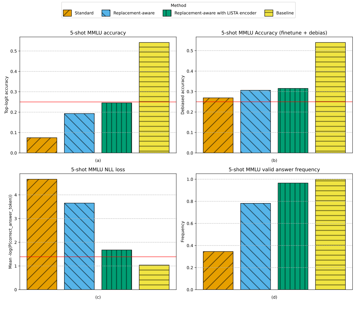
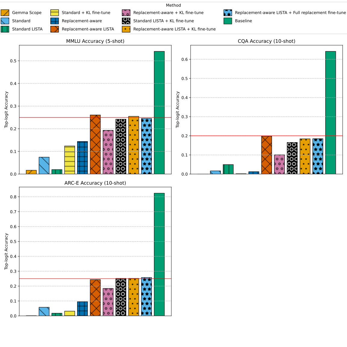
- These reductions in KL divergence matter qualitatively. My replacement models retain some degree of capability as measured by benchmarks like MMLU, whereas alternatives do not remain coherent enough to even reliably give valid answers on these tasks.
2 Background
In this section I set up a notational framework for explaining my methods and how they differ from existing approaches. I also briefly outline my case against error nodes.
2.1 Replacement models
A replacement model is a modification to a transformer model in which some subset of internal activations are re-encoded as a sparse sum of interpretable features. In this post I will focus on replacement models using SAEs that operate on the residual stream, though these methods should also be applicable to finer-grained replacement models. For precision I will use the term \(r\)-replacement model, denoted \(\widehat{M}^r\), where \(r \subseteq[0..m-1]\), to specify which layers’ residuals have been re-encoded. Note that this distinction between different replacement models is the defining difference between replacement-aware training and existing methods. I’ll refer to the \([0..m-1]\)-replacement model as the full replacement model, while the \(\emptyset\)-replacement model is simply the base model. Formally, letting \(P\) be the function converting the final residual to probabilities, \(m\) the number of layers, \(\mathrm{SAE}_i\) an SAE trained on the \(i^{th}\) layer’s residual, \(T_i\) the \(i^{th}\) transformer layer, and \(x\) the embedding of an arbitrary input, define the \(r\)-replacement model as
\[ \begin{gather} \widehat{M}^r(x) = P \circ \widehat{T}^r_{m-1} \circ \widehat{T}^r_{m-2} \circ \dots \circ \widehat{T}^r_0(x) \\ \widehat{T}^r_i=\cases{ \mathrm{SAE}_i \circ T_i & if $i \in r$ \\ T_i & otherwise. } \end{gather} \tag{1}\]
In this post I will explore variant encoder designs while keeping the decoder step a simple affine transformation. Hence, with \(E_i:\mathbb{R}^{d_{model}}\rightarrow \mathbb{R}_+^{d_{sae}}\) the encoder function mapping activations to features, we have
\[ \begin{align} \mathrm{SAE}_i(a)&=D_i \circ E_i(a)\\ D_i(x)&=x(W_i^{dec})^T+b_i^{dec}, \end{align} \tag{2}\]
where \(W_i^{dec} \in \mathbb{R}^{d_{model} \times d_{sae}}\) and \(b_i^{dec} \in \mathbb{R}^{d_{model}}\) are the decoder (or dictionary) weights and biases for the \(i^{th}\) layer SAE.
We’ll also find it convenient to refer to the activations of the \(i^{th}\) layer in a replacement model
\[ \begin{align} \widehat{A}^r_i(x)=\widehat{T}^r_i\circ\widehat{T}^r_{i-1}\circ \dots \circ \widehat{T}^r_0(x) \end{align} \tag{3}\]
as well as the SAE features
\[ \begin{align} \widehat{F}^r_0(x) = E_0 \circ T_0(x) \\ \widehat{F}^r_i(x) = E_i \circ T_i \circ\widehat{T}^r_{i-1}\circ \dots \circ \widehat{T}^r_0(x). \end{align} \tag{4}\]
Note that the features for SAE \(i\) are defined by Equation 4 even when \(i \notin r\). Note also that these definitions imply that activations and features for layer \(i\) are not affected by the inclusion or exclusion of \(j>i\) in the replacement set:
\[ \begin{align} \widehat{A}^{r\subseteq[0..i]}_i&= \widehat{A}^{r\cup\{j | j > i\}}_i = \widehat{A}^{r \cup [i+1..m-1]}_i\\ \widehat{F}^{r\subseteq[0..i]}_i&= \widehat{F}^{r\cup\{j | j > i\}}_i = \widehat{F}^{r \cup [i+1..m-1]}_i, \end{align} \]
so I will use these interchangeably when notationally convenient. The relationships among these terms are visualized as a causal graph below.
2.2 Error nodes
In the introduction, I claimed that replacement models using more than a few SAEs become entirely incoherent. It might not be intuitively obvious how bad the problem is from just looking at plots of KL divergence. Thus, I think it’s illustrative to compare actual rollouts from different replacement models. Note especially that the naive Gemma Scope output is not recognizable as language:
Effect of sleep quality on memory, executive function, and language performance in patients with refractory focal epilepsy and controlled epilepsy versus healthy controls - A prospective study. We aimed to evaluate the effect of sleep quality on memory, executive function, and language performance … Shorter total sleep time, poorer sleep efficiency, and prolonged sleep latencies were observed to be associated with poor memory and executive function in patients with refractory epilepsy.
Gemma Scope
//_//_// //ing
Gemma Scope with encoder tuning
The results of this study suggest that the effect of
Replacement-aware
The results suggest that the sleep quality of patients with
Base model
<b>BACKGROUND:</b> The aim of this study
True continuation
Our study strongly suggests that sleep disturbances, mainly
Recognizing this issue, Marks et al. (2024) account for the errors introduced by SAEs in the replacement model by adding an additional term that exactly cancels them out. They refer to these terms as error nodes, as they are incorporated into the computational graph that is the basis of their circuit discovery method. Translated to the nomenclature of this post, this looks like:
This style of error node has become somewhat of a standard practice in feature-based circuits work; see for example (Ge et al. 2024; Ameisen et al. 2025; Hanna et al. 2025; Yang et al. 2026). One widely acknowledged limitation of this approach is that causal effects attributed to such nodes are inherently uninterpretable, and in some cases dominate the recovered circuits (Ameisen et al. 2025). A further drawback is that this is incompatible with learning-based approaches to circuit discovery, since the error node removes any incentive for more accurate reconstruction; see the discussion in \(\S 2.3.3\) of Caples et al. (2025). However, I believe there is a more fundamental issue with this approach: while it successfully builds consistent representations for observational data, it breaks down once we start trying to apply it to causal interventions. I relegate the full argument to Appendix C.1, since it is immaterial to my empirical results, but to briefly summarize:
- Because each error node value is precisely tuned to cancel out the reconstruction error, its effects are different depending on whether we have intervened on any features.
- This results, post-intervention, in a computational pathway with values depending on serial reconstructions, the very situation the error nodes were trying to prevent.
- This is in fact an unavoidable consequence of feature space interventions, because such a pathway is the only possible mechanism by which these interventions could have any counterfactual implications.
The situation is more complicated for the attribution graphs of Ameisen et al. (2025) due to the use of CLTs rather than SAEs, resulting in many additional pathways that could potentially overwhelm the effect described above. Even so, most of these paths contain serial reconstructions of varying length: \(m-i \over 2\), on average, for the effect of an intervention at layer \(i\) on the final layer.1 This might explain the observation that effective steering magnitudes had to be guessed and checked, rather than falling directly out of the model. If this argument holds, then to get feature circuits that are capable of making accurate causal predictions such as the effects of steering, we must address the problem of compounding error head-on. The remainder of this post is my attempt to do exactly that.
3 Methods
Three core innovations underlie my improved replacement model: replacement-aware training, encoder fine-tuning, and a more powerful encoder inspired by LISTA (Gregor and LeCun 2010). I outline each below.
3.1 Replacement-aware training
Standard SAE training methods deal with each SAE in isolation. Even though end-to-end training (Braun et al. 2024) includes terms for downstream reconstruction errors, it still uses only one SAE in its replacement model. This approach can be glossed in my terminology as2
\[ \begin{array}{rcl} \mathscr{L}^{e2e}_i & = & \alpha_1 \cdot \mathrm{KL}(\widehat{M}^{\{i\}}(X)\;\|\;\widehat{M}^{\emptyset}(X)) \\ & + & \alpha_2 \cdot \displaystyle\sum\limits_{\ell=i+1}^{m-1} \mathrm{MSE}(\widehat{A}^{\{i\}}_\ell(X),\; \widehat{A}_{\ell}^{\emptyset}(X)), \end{array} \tag{5}\]
where \(X\) is a batch of inputs.
In contrast, replacement-aware training uses a replacement model in which additional downstream layers are also replaced with the corresponding SAE outputs. Note that this implies a serial ordering to SAE training; we must have trained layers \([i+1..m-1]\) before we train the SAE for layer \(i\). In the most general form, the loss function for replacement-aware training is given by
\[ \begin{array}{rcl} \mathscr{L}^{ra}_i & = & \alpha_1 \cdot \mathrm{KL}(\widehat{M}^{[i..m-1]}(X)\;\|\; \widehat{M}^{\emptyset}(X)) \\ & + & \alpha_2 \cdot \sum\limits_{\ell=i}^{m-1} L_\ell(\widehat{F}^{[i..m-1]}_\ell(X),\; \widehat{F}_\ell^{\emptyset}(X)), \end{array} \tag{6}\]
where \(L_\ell\) are functions of the SAE features in the replacement model starting at the current layer versus those that would have been computed from base model activations. The MSE on the SAE reconstructions is one such function, but in informal experiments I got slightly better results using the cosine distance on the features themselves. I also found that simply using the next layer (i.e. letting \(L_\ell=0\) for \(\ell>i+1\)) rather than all downstream layers was sufficient for greatly improved performance. The intuition behind only including the next layer is that, due to the serial layout of the transformer blocks, the output of the next layer screens off any influence the current layer could have on the later blocks3. I view this term as a regularization that penalizes the SAE for destroying information that is useful downstream, even if it may not be relevant for the current layer. Since the next layer’s features were also trained with this objective, this argument hypothetically chains all the way forward to the logits, so we are effectively implementing an approximation to end-to-end training of the full replacement model.
Additionally, to save on compute, I only include the \(KL\) term on the final layer, treating the logits as a virtual “next layer”. For earlier layers, I run a separate KL fine-tuning stage for the final 20% of training tokens, similarly to Karvonen (2025). This allows its impact to be easily disentangled from that of replacement-aware training itself. I tried a few variants of this stage using different subsets of the downstream replacement model, which I’ll describe below.
For all results in this post labeled “replacement-aware training”, the main phase of training uses the loss function
\[ \begin{array}{rcl} \mathscr{L}^{nl}_{m-1} & = & \alpha_1 \cdot \mathrm{MSE}(\widehat{A}^{\{m-1\}}_{m-1}(X),\ \widehat{A}^{\emptyset}_{m-1}(X)) \\ & + & \alpha_2 \cdot \mathrm{KL}(\widehat{M}^{\{m-1\}}(X) \;\|\; \widehat{M}^{\emptyset}(X)) \\ \mathscr{L}^{nl}_{i\in[0..m-2]} & = & \alpha_1 \cdot \mathrm{MSE}(\widehat{A}^{\{i,i+1\}}_i(X),\ \widehat{A}^{\emptyset}_i(X)) \\ & + & \alpha_2 \cdot \mathrm{cosdist}(\widehat{F}^{\{i, i+1\}}_{i+1}(X),\ \widehat{F}^{\emptyset}_{i+1}(X)), \end{array} \tag{7}\]
which is simply the standard SAE loss function rendered in my notation, with an additional term penalizing distortions to the next layer’s SAE features, or, in the case of the final layer, KL divergence from the base model. Note that the weights of \(\mathrm{SAE}_{i+1}\) are frozen before starting training on \(\mathrm{SAE}_i.\) After Karvonen (2025), the weights \(\alpha_1, \alpha_2\) are set per-batch such that the total magnitudes of the corresponding terms match. Standard training is equivalent to setting \(\alpha_2\) to 0.
3.1.1 KL fine-tuning
For the fine-tuning stage, we’ll consider three variants: standard KL fine-tuning (Karvonen 2025), next-layer fine-tuning, and full replacement fine-tuning. Standard KL fine-tuning is simply
\[ \begin{array}{rcl} \mathscr{L}^{kl}_i & = & \alpha_1 \cdot \mathrm{MSE}(\widehat{A}^{\{i\}}_i(X),\ \widehat{A}^{\emptyset}_i(X)) \\ & + & \alpha_2 \cdot \mathrm{KL}(\widehat{M}^{\{i\}}(X)\;\|\;\widehat{M}^{\emptyset}(X)). \end{array} \tag{8}\]
Next-layer fine-tuning is identical to Equation 7 for the final layer; for other layers a third term for the \({\{i,i+1\}}\)-replacement KL is added:
\[ \begin{array}{rcl} \mathscr{L}^{nlf}_{i\in[0..m-2]} & = & \alpha_1 \cdot \mathrm{MSE}(\widehat{A}^{\{i,i+1\}}_i(X),\ \widehat{A}^{\emptyset}_i(X)) \\ & + & \alpha_2 \cdot \mathrm{cosdist}(\widehat{F}^{\{i, i+1\}}_{i+1}(X),\ \widehat{F}^{\emptyset}_{i+1}(X))\\ & + & \alpha_3 \cdot \mathrm{KL}(\widehat{M}^{\{i,i+1\}}(X) \;\|\; \widehat{M}^{\emptyset}(X)). \end{array} \tag{9}\]
Finally, full-replacement fine-tuning is equivalent to Equation 9, but the full replacement model starting at layer \(i\) is used. Note that this method is substantially more expensive to run in terms of both memory and compute. I also found it to be much less stable; training runs diverged unless I performed encoder tuning (Section 3.2) beforehand, which makes it harder to compare to other methods. However, I include it here since it resulted in my best-performing replacement model:
\[ \begin{array}{rcl} \mathscr{L}^{fr}_{i\in[0..m-2]} & = & \alpha_1 \cdot \mathrm{MSE}(\widehat{A}^{[i..m-1]}_i(X),\ \widehat{A}^{\emptyset}_i(X)) \\ & + & \alpha_2 \cdot \mathrm{cosdist}(\widehat{F}^{[i..m-1]}_{i+1}(X),\ \widehat{F}^{\emptyset}_{i+1}(X))\\ & + & \alpha_3 \cdot \mathrm{KL}(\widehat{M}^{[i..m-1]}(X) \;\|\; \widehat{M}^{\emptyset}(X)) \end{array} \tag{10}\]
As before, the \(\alpha_j\) weights are adjusted per-batch so that all terms have the same magnitude.
3.2 Encoder tuning
Extracting features from model activations is fundamentally an inference problem. The way we go about this need not be grounded in concrete model mechanisms, because by hypothesis the model’s actual computation takes place in the smaller, superimposed space. In other words, while the decoding step of an SAE must be constrained by observable model behavior, we have flexibility in defining the encoder. We can use this freedom to build in robustness to the errors introduced by upstream SAEs in the replacement model.
Specifically, I propose an additional training stage that takes each layer’s SAE decoder as fixed, tuning the encoder such that its output in the replacement model more closely matches its output on the base model, while also minimizing distortions to the next layer’s features. Let \(\mathrm{SAE}_{pre,i}\) be a set of SAEs defined as in Equation 2, and initialize a matching set of \(\mathrm{SAE}_{post,i}\) with these parameters. Then, proceeding in ascending layer order4, optimize the encoder parameters of each \(\mathrm{SAE}_{post,i}\) according to
\[ \begin{array}{rcl} \mathscr{L}_{i \in[0..m-2]}^{et} & = & \alpha_1 \cdot \mathrm{MSE}(\widehat{F}^{[0..i]}_{post,i}(X), \widehat{F}^{\emptyset}_{pre,i}(X)) \\ & + & \alpha_2 \cdot \mathrm{MSE}(\widehat{F}^{[0..i+1]}_{post,i+1}(X),\widehat{F}^{\emptyset}_{pre,i+1}(X)) \\ \mathscr{L}_{m-1}^{et} & = & \alpha_1 \cdot \mathrm{MSE}(\widehat{F}^{[0..m-1]}_{post,m-1}(X),\widehat{F}^{\emptyset}_{pre,m-1}(X)) \\ & + & \alpha_2 \cdot \mathrm{KL}(\widehat{M}^{[0..m-1]}_{post}(X)\;\|\;\widehat{M}^{\emptyset}(X)). \end{array} \tag{11}\]
The rationale for freezing the decoders is that the dictionaries learned at each layer were optimized for base model activations, which is a property we want to preserve; that’s the entire reason we expect them to have any bearing on reality! As for the ordering: in the full replacement model, we are now running the SAEs off-distribution, with the exception of layer 0, since there is nothing to distort its input. By first tuning the layer 0 encoder, we bring the layer 1 encoder’s input closer to its training distribution. Fixing the result and tuning the layer 1 encoder then aligns the input of the layer 2 encoder; and so on through the rest of the model.
Note that this procedure can be run on any set of SAEs, replacement-aware or not, and this offers substantially improved performance in the replacement model even with very short training runs, on the order of 1 million tokens.5 I applied this procedure to all the SAEs discussed in this post to provide a fairer comparison.
3.3 Encoder variants
3.3.1 BatchTopK
The standard SAE computes features with a single linear operation followed by a nonlinear activation function. Several activation functions are in common use, but for this post I will be using BatchTopK (Bussmann et al. 2024), which is effectively a JumpReLU (Rajamanoharan et al. 2024) with a single global threshold. During training, a BatchTopK encoder computes features for a batch of \(n\) tokens by keeping the top \(k \cdot n\) values after the linear transform and setting the rest to 0. My implementation is a very slight tweak to this, in that I always operate the function as a JumpReLU but with the threshold adaptively chosen to match the chosen sparsity as closely as possible, while enforcing non-negativity6:
\[ \begin{aligned} F_i^{btk}(a) &= h^{btk(k)}(Y_i(a))\\ h^{btk(k)}(y)[t] &= \left\{ \begin{array}{lr} y[t], & y[t] \geq \max(0, \mathrm{topk}(y, k\cdot n)) \\ 0, & \text{ otherwise} \end{array} \right. \\ Y_i(a) &= a(W^{enc}_i)^T + b^{enc}_i . \end{aligned} \tag{12}\]
\(k\) is a hyperparameter controlling the desired sparsity and \(W_i^{enc} \in \mathbb{R}^{d_{sae} \times d_{model}}\) and \(b_i^{enc} \in \mathbb{R}^{d_{sae}}\) are the encoder weights and bias. At inference time, this can be instead used as a JumpReLU:
\[ F_i^{jr}(a)[t] = \left\{ \begin{array}{lr} Y_i(a)[t] & Y_i(a)[t] \geq \theta_i \\ 0 & \text{otherwise,} \end{array}\right . \tag{13}\]
where \(\theta_i\) is a threshold learned during training7 such that the expected sparsity matches the target.
3.3.2 LISTA
LISTA (Gregor and LeCun 2010) is an approach to sparse coding based on “unrolling” the classic ISTA algorithm (Daubechies et al. 2004) into a neural network. LISTA treats the matrices used to iteratively update the estimated sparse representation as learnable parameters; each iteration of the original algorithm is then represented by a single layer of a neural network. Translating the original presentation into the parlance of the current post, LISTA with \(n_{iter}\) iterations computes the following features:
\[ \begin{gather} F_i(a)=z^{n_{iter}}_i(a) \\ z^0_i(a)=0 \\ z^{j+1}_i(a)=h^j_i(a(W^{enc}_i)^T + S_iz^{j}_i(a)), \end{gather} \tag{14}\]
where \(S_i \in \mathbb{R}^{d_{sae} \times d_{sae}}\) is termed the mutual inhibition matrix and \(h^j_i\) is an activation function, which we will allow to vary per-iteration and per-layer.8 Note that when \(n_{iter}=1\) this is exactly equivalent to a vanilla SAE with \(b_i^{enc}=0\).
One major drawback of applying this directly as an SAE encoder is the number of parameters, which is now \(O(d_{sae}^2),\) much larger than a standard SAE with \(O(d_{sae}\cdot d_{model}),\) since typically \(d_{sae} \gg d_{model}.\) Fortunately, subsequent work brings this down to be in line with standard SAEs. Chen et al. (2018) argue for a weight-coupling scheme that effectively removes the parameter \(S_i\), but also add separate \(W^{enc,j}_i\) weights for each iteration, resulting in \(O(d_{sae}\cdot d_{model} \cdot n_{iter})\) total parameters. Liu et al. (2019) build on this further, showing that the per-iteration weights can actually be taken to be scalar multiples of each other, resulting in a final parameterization that is just \(O(d_{sae}\cdot d_{model})\); this is just the standard SAE encoder weights, plus \(n_{iter}\) scalars, which is negligible in comparison.
Chen et al. (2018) also propose what is effectively a “firm shrinkage” (Gao and Bruce 1997) activation function in place of the standard soft shrinkage. Specifically, the top \(k\) inputs (in absolute value) are passed through unchanged, while the rest are subject to the standard soft shrinkage function. If we drop the soft shrinkage part, this is just the familiar TopK activation function! Putting this all together, swapping in BatchTopK in place of TopK, and adding the “Onsager correction” term from Borgerding and Schniter (2016) for improved stability, results in
\[ \begin{align} F_i^{LISTA}(a) &= z^{n_{iter}}_i(a) \\ z_i^0(a) &= 0 \\ r_i^0(a) &= a - D_i(z_i^0(a)) \\ r_i^{j+1}(a) &= a - D_i(z_i^{j}(a)) + k_j \cdot r_i^{j}(a) / d_{model}\\ z_i^{j+1}(a) &= h_i^{btk(k_j)} \left (z_i^{j}(a) + \gamma_i^j \cdot r_i^{j+1}(a)(W_i^{enc})^T \right ). \end{align} \tag{15}\]
For this post, I used \(k_j=((j+1)\cdot \frac{k_{max}}{n_{iter}})\), i.e. stepping up \(k\) in equal increments, specifically [20, 40, 60, 80, 100]. This is a similar scheme to that used in \(LISTA{\text -}SS\) from Chen et al. (2018). \(D_i\) is the standard SAE decoder from Equation 2, and \(\gamma_i^j\) are the per-iteration scalar factors from Liu et al. (2019). For improved stability—I often observed feature values exploding once the SAE was off-distribution, as happens when using it in the replacement model—I additionally apply PyTorch’s spectral norm parameterization to the encoder weight matrix and soft-cap the scalars \(\gamma_i^j\) to a max of 1 with tanh. This probably isn’t the best way of dealing with the instability, but it was sufficient to get consistently well-behaved training runs for a 5-iteration variant. I leave optimizing the exact setup to future work.
I think once we write down LISTA this way, the way it works is fairly intuitive: we simply pass the current residual \(a - D_i(z_i^j)\) plus the Onsager correction \(k_j\cdot r_i^j/d_{model}\) (which is effectively a skip connection from the previous iteration) into the encoder, repeatedly. Because \(k\) increases with each iteration, this means that additional features are selected conditional on the ones that have been already added. This could allow the SAE to handle hierarchical structure within the features, as has been proposed in prior work (Costa et al. 2025; Bussmann et al. 2025). Indeed, with sufficient hand-waving one could view this process as an approximation to (a learned version of) matching pursuit (Mallat and Zhang 1993), where due to the increasing \(k\) for the BatchTopK activation functions, we are selecting \(\frac{k_{max}}{n_{iter}}\) new features per iteration instead of just 1.
4 Results
In this section I first present my core results, then investigate the individual contributions of each of my methods. I describe the training process in more detail in Appendix A.1. Source code is available on GitHub. Data, including all SAE weights, validation and benchmark results, and tables and plots included in this post are available via huggingface bucket; see previous GitHub link for an explanation of the directory layout.
All results presented here are based on complete sets of SAEs I trained on all 26 layers of Gemma-2-2B in various configurations, using between 50 and 100 million tokens from the pile-uncopyrighted (Gao et al. 2020) training split per layer. The core training pipeline consists of 3 stages: initial training (Section 3.1), KL fine-tuning (Section 3.1.1), and encoder tuning (Section 3.2). I found that performing KL fine-tuning with the full replacement model (Equation 10) was much less stable than using the this-and-next-layer-only replacement model (Equation 9), in addition to requiring much more memory (and thus more expensive hardware to achieve reasonable training times for 26 SAEs). While interchanging the order of this step with encoder tuning did mitigate this somewhat, doing so also makes it impossible to perform some of the analysis I want to show later in the results. Thus, I restrict the use of Equation 10 to a single “flagship” model, which I will exclude from the comparisons it is incompatible with.
To investigate how changes to the training setup and encoder design impact the end-to-end performance of the full replacement model, I trained using all configurations from the cross product
(standard main phase, next-layer main phase)
\(\times\) (no KL fine-tuning, KL fine-tuning on 10 million tokens)
\(\times\) (“vanilla” SAE encoder, 5-iteration LISTA encoder)
For KL fine-tuning, I matched the loss to the corresponding main phase method, so that results labeled “standard” used Equation 8 and ones labeled “replacement-aware” used Equation 9. The amount of total training data varied because after my initial runs of 100 million tokens (which happened to be for vanilla next layer), looking at the loss history revealed severely diminishing returns after about 50 million tokens, so I shortened the runs that came after that analysis to save on compute costs. Below is a summary table of the SAEs, along with links to their weights:
| Weights | Main training phase | KL fine-tune phase | Encoder |
|---|---|---|---|
| Encoder-tuned Pre-tuning |
Standard, 5e7 tokens | None | Vanilla BatchTopK, k=100 |
| Encoder-tuned Pre-tuning |
Standard, 5e7 tokens | 1e7 tokens | Vanilla BatchTopK, k=100 |
| Encoder-tuned Pre-tuning |
Standard, 5e7 tokens | None | LISTA BatchTopK, k=[20, 40, 60, 80, 100] |
| Encoder-tuned Pre-tuning |
Standard, 5e7 tokens | 1e7 tokens | LISTA BatchTopK, k=[20, 40, 60, 80, 100] |
| Encoder-tuned Pre-tuning |
Next layer, 1e8 tokens | None | Vanilla BatchTopK, k=100 |
| Encoder-tuned Pre-tuning |
Next layer, 9e7 tokens | 1e7 tokens | Vanilla BatchTopK, k=100 |
| Encoder-tuned Pre-tuning |
Next layer, 5e7 tokens | None | LISTA BatchTopK, k=[20, 40, 60, 80, 100] |
| Encoder-tuned Pre-tuning |
Next layer, 5e7 tokens | 1e7 tokens | LISTA BatchTopK, k=[20, 40, 60, 80, 100] |
| Encoder-tuned (no pre-tuned version available) |
Next layer, 5e7 tokens | 1e7 tokens, full replacement (Equation 10) | LISTA BatchTopK, k=[20, 40, 60, 80, 100] |
Since these SAEs were trained using my own choice of hyperparameters and code, which could be buggy, as a sanity check I also compared them to the Gemma Scope (Lieberum et al. 2024) residual stream SAEs, using encoder tuning (Section 3.2) to match their sparsity to my SAEs. See Appendix A.4 for further details.
4.1 Headline results
Applying my full method results in replacement models with greatly improved end-to-end performance compared to standard approaches. Below, I plot an expanded version of Figure 1 on 1 million tokens from the pile-uncopyrighted (Gao et al. 2020) validation split for the full suite of SAEs that I studied. Note that I report geometric means, rather than arithmetic means, because this is a more appropriate summary statistic given the per-token distribution of these values.9 Note also that all SAEs in this chart are post encoder tuning, due to this having a disproportionate impact on the worst-performing replacement models. I explore this effect in more detail in Section 4.4.
| Loading ITables v2.8.0 from the internet... (need help?) |
To put these numbers into context, I also compared performance on the question-answering benchmarks MMLU (Hendrycks et al. 2020), CommonsenseQA (CQA) (Talmor et al. 2018), and the ARC Easy set (ARC-E) (Clark et al. 2018). I chose these benchmarks primarily for ease of implementation, since their data are readily available and evaluation only requires computing logits for single tokens, and because they offer a range of difficulties for the base model (54% accuracy for MMLU, 64% for CQA, 82% for ARC-E). See Appendix A.2 for details on the exact prompting setup I used.
| Loading ITables v2.8.0 from the internet... (need help?) |
Disappointingly, no method consistently breaks chance performance, despite clear improvements resulting from the combination of replacement-awareness, KL fine-tuning, and using LISTA encoders. Investigating further, I found that these differences are largely driven by some replacement models’ (in)ability to even give a valid answer to a multiple-choice question, and a marked propensity for particular responses even when they are valid:
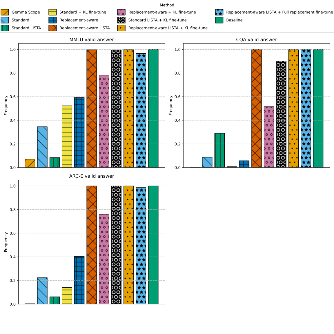
| Loading ITables v2.8.0 from the internet... (need help?) |
So far, it appears that improved replacement models are able to recover some degree of in-context learning, to the extent that they can at least consistently recognize when a multiple-choice answer is required, but then they hit a ceiling. These tasks are likely being made more difficult by the relatively poor generalization of SAEs outside of the distributions they were trained on (Kissane et al. 2024; Heindrich et al. 2025). To mitigate this, I re-ran KL fine-tuning (Section 3.1.1) for the methods that included that step while interleaving a mix of questions and answers from the CQA train split.10 Specifically, 10% of tokens were from variable-length examples matching the n-shot template used in benchmarking (see Appendix A.3) and 90% were from pile-uncopyrighted (as in all other training runs). Since the fine-tuning step is 20% of the total token budget, this affects 2% of the total training data. Additionally, to mitigate the bias observed in Table 6, I applied PriDe (Zheng et al. 2023), which estimates and adjusts for a question-independent prior probability on each label by augmenting the dataset with additional copies of a subset of examples with their options permuted. Note that this implicitly uses the probabilities of responses conditioned on the answer being valid, so this isn’t quite directly comparable to the previous plot, at least for the Standard replacement model. However, since fine-tuning saturated the valid response fraction for the other methods (see second tab), this is directly comparable for them.
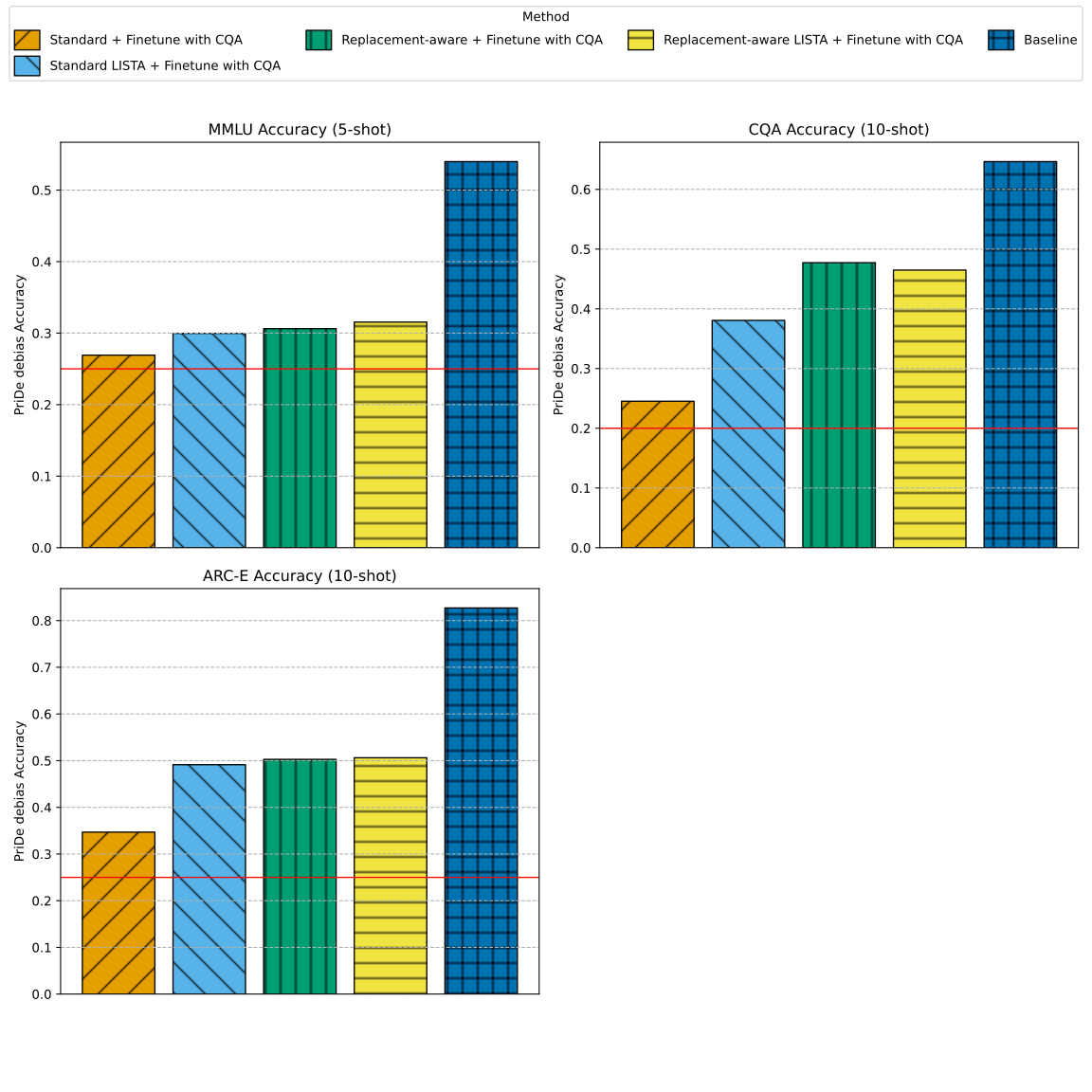
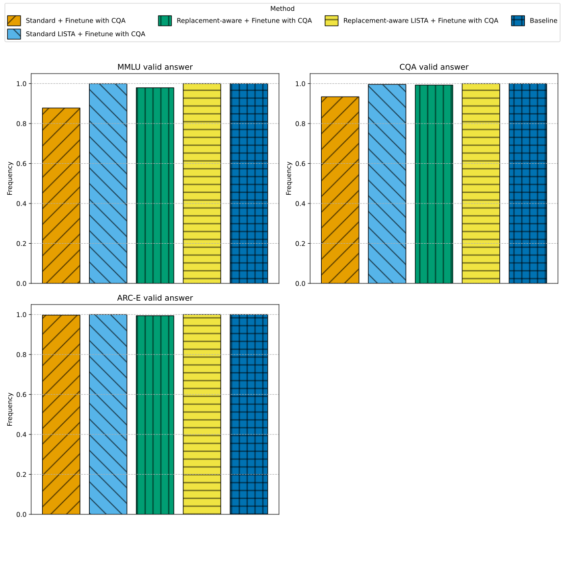
| Loading ITables v2.8.0 from the internet... (need help?) |
These plots show a clear advantage for both replacement-aware training and the LISTA encoder, but no apparent additional benefit for their combination. In the following, I will explore the individual effects of each of these variants.
4.2 Replacement-aware training does not sacrifice faithfulness
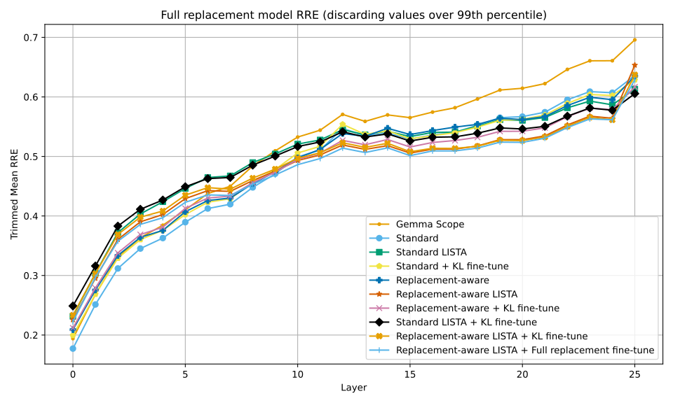
Another important metric to consider is the quality of the SAE reconstructions. Because SAEs are learned, it is possible that they pick up on patterns that aren’t actually used by the underlying model. Their utility as explanations of model behavior is thus contingent on their representations being grounded in the true activations; they should be faithful. To measure this, I report the relative reconstruction error (RRE)11, defined as \(\mathrm{RRE}(X, Y)=||X - Y||_2/||Y||_2\), averaged across 1 million validation tokens. Note that I am plotting trimmed means (arithmetic means calculated with values in the \(99^{th}\) percentile and above discarded) to deal with extreme outliers for some methods. Note also that methods using the LISTA encoder don’t have this outlier problem, which may be noteworthy in and of itself; see the table of un-trimmed arithmetic means below.
| Loading ITables v2.8.0 from the internet... (need help?) |
| Loading ITables v2.8.0 from the internet... (need help?) |
I notice a couple of noteworthy aspects of this chart. First, the overall shape is very similar across all methods. We’ll investigate the specific shape shortly, but I’d like to also call attention to the region between layers 5 and 10. At earlier layers, standard training outperforms replacement-aware methods, but the lines cross over somewhere in this region and stay that way until the final layer. To make this clearer, here’s the same plot limited to just standard training and the best-performing replacement-aware version:
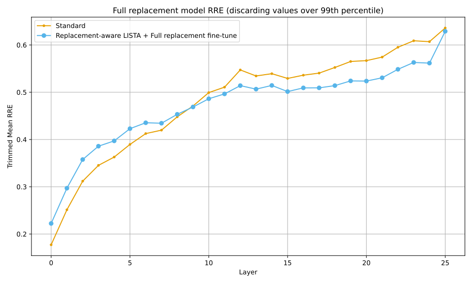
In fact, replacement-aware training seems to be comparable or even strictly better by this metric when compared with its replacement-naive counterparts:
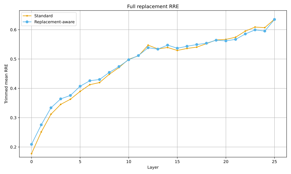


With the exception of the non-finetuned standard encoder, where the values are essentially equal past the early layers, we actually see lower RRE when using replacement-aware training. In other words, replacement-aware training is not sacrificing faithfulness to achieve its improved end-to-end performance!12
4.3 A simple model of reconstruction error
The reconstruction error of each SAE, considered in isolation, has been a primary metric for almost all prior work on SAEs for mechanistic interpretability. But I don’t think it makes sense to consider the SAEs in isolation; a good representation needs to capture all relevant information, where “relevance” includes sufficiency for constructing accurate downstream representations. As I just showed in the previous section, replacement-aware training is superior to standard training in this regard. As might be expected from the form of Equation 7, which is the standard SAE objective plus an additional term, this trades off against the traditional metric. As I’ll show in this section, the primary advantage of replacement-aware training is a reduction in the compounding effect of SAE error, which grows with model depth.
Let’s now return to the shape of Figure 10. A straightforward model of reconstruction error is to consider two sources: error caused by an intrinsic “difficulty level” of sparse coding at each layer, and a second-order effect caused by the reconstruction target itself being offset from the true activations. While we could in principle quantify the first effect by estimating the entropy of the high-dimensional joint distribution of activations at each layer, we already have a much more convenient proxy. Prior to encoder tuning, every SAE was trained with an objective that included the MSE for the current layer against the true activations. We should thus expect the reconstruction performance in the single-SAE-on-baseline-activations case to be inversely proportional to the underlying difficulty, modulo some offset due to MSE trading off against other objectives for some methods. And indeed, we see essentially the same shape across all the methods I tested:
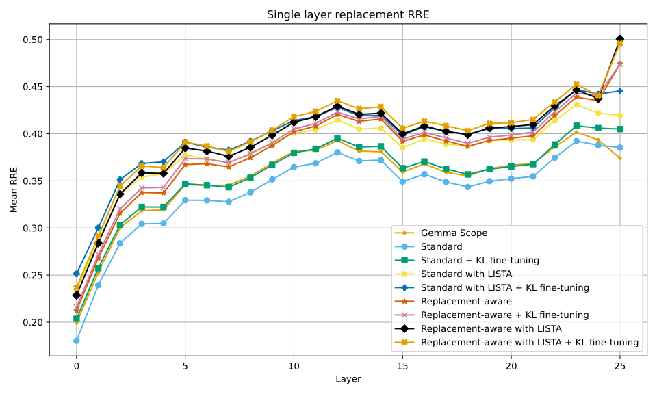
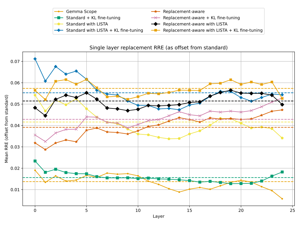
| Loading ITables v2.8.0 from the internet... (need help?) |
To account for the second-order effect, a naive model would be to assume that the additional error is additive and independent. This would imply growth proportional to the square root of depth, since we’re in high enough dimensions that randomly selected error directions will be orthogonal to each other. That is, if \(\eta_i\ \mathrm{s.t.}\ ||\eta_i||_2 \leq c\) is the error added at layer \(i\), then the magnitude of the total error under this model for the \(i^{th}\) layer would be given by
\[ ||\epsilon_i||_2 \approx \sqrt{\sum_{j\leq i}{||\eta_j||^2_2}} \leq c\cdot\sqrt{i+1}. \tag{16}\]
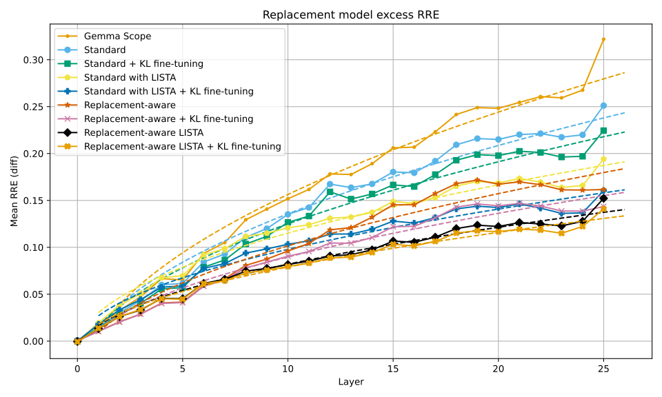
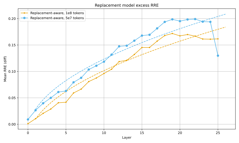
While this is almost certainly overly simplistic, if we plot the excess error in the full replacement model over the corresponding single-SAE error along with a best-fit square root, we can see that it fits remarkably well, at least once we get about a third of the way through the model:
| Loading ITables v2.8.0 from the internet... (need help?) |
| Loading ITables v2.8.0 from the internet... (need help?) |
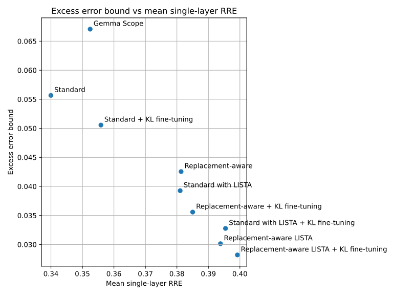
I propose, then, that one way to understand the effectiveness of an SAE training method is to consider this limiting constant as a measure of how quickly re-encoding error compounds. To what extent it is worth trading off individual layer accuracy to decrease the bound depends on the depth of the model in question. This certainly makes it more challenging to validate potential improvements, since they may not even be measurable until you’ve already trained many SAEs with them, and toy models may be too shallow to even observe a difference! Empirically, as we saw in Figure 11, in Gemma-2-2B this trade-off only becomes beneficial after 9 layers, even for my best-performing method. I suspect that truly optimizing end-to-end replacement model performance will require a deeper understanding of how and why certain representations generalize better, such that one can iterate on the training setup without having to train a full replacement model as I needed to here.
Visualizing the error bound versus the single-layer RRE in a Pareto frontier-ish13 way shows that replacement-awareness, KL fine-tuning, and LISTA all push in the direction of making more of the trade-off of individual layer accuracy for slower error compounding:
| Loading ITables v2.8.0 from the internet... (need help?) |
4.4 Encoder tuning is effective
Encoder tuning (Section 3.2) appreciably improves replacement model performance. While the impact is greatest on replacement-naive SAEs, this effect does stack with the improvements from replacement-aware training:
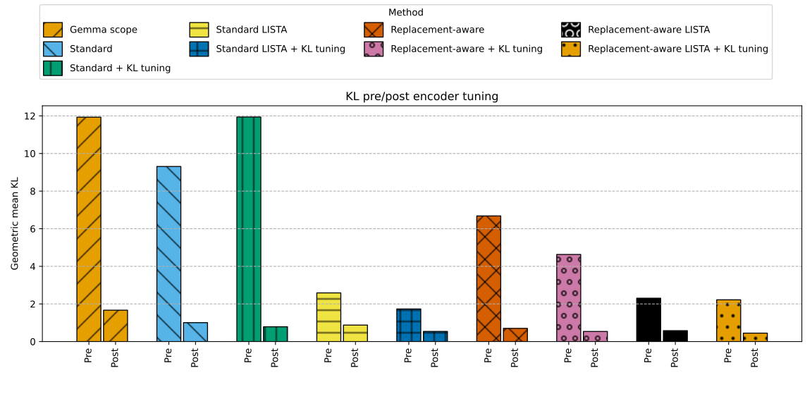
It’s worth exploring how such a short fine-tuning stage can have such a large impact. One potential cause is the fact that error induced by the replacement model in early layers has a big effect on the statistics of the activations reaching later layers. The SAEs used here are especially sensitive to this due to the threshold parameters in their activation functions. Although replacement-aware training attempts to minimize such distortions, each SAE was still trained with inputs coming entirely from the base model distribution. One major function of encoder tuning is to adapt these thresholds to the new statistics, which we can see is effective by comparing feature \(L_0\) stats before and after this phase:
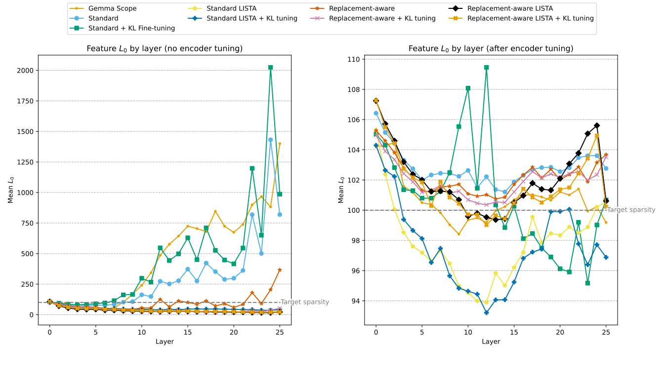
Does this fully explain the effectiveness of encoder tuning, or is there additional impact of fine-tuning the other encoder parameters? Because these SAEs use the BatchTopK activation function14, we can check this directly by comparing performance for the tuned variants versus the pre-tuned versions with their adaptive “training mode” thresholds. Evidently, there is some additional effect of tuning the full set of parameters, though this ranges from a quite large effect for Gemma Scope to a negligible one for the LISTA and replacement-aware SAEs:
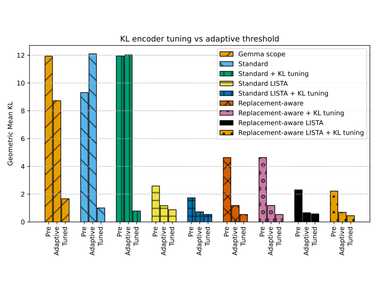
This isn’t definitive, but these results could be evidence that the LISTA/replacement-aware SAEs were already mostly adapted to the replacement model, modulo the activation statistics. In contrast, the standard SAEs had more room for improvement and so fine-tuning the encoder parameters had a much greater impact. It might be worth investigating encoder tuning as a standalone method, since it is applicable independently of any initial training.
4.5 KL fine-tuning doesn’t degrade reconstruction quality
Since I use KL fine-tuning extensively, it’s worth quickly sanity checking that it doesn’t degrade reconstruction quality. If we pair methods by whether or not they included this phase, we see that they are indeed very close:
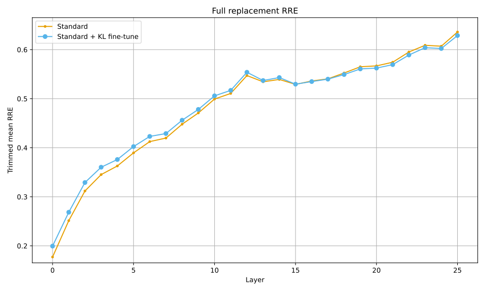
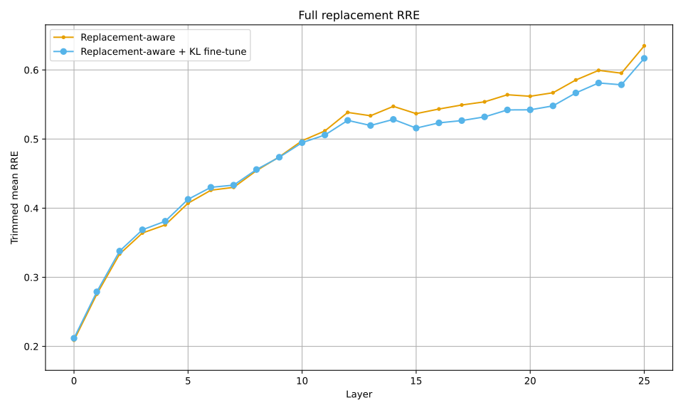


4.6 LISTA encoders improve robustness to upstream error
We have already seen that using the LISTA encoder improves end-to-end performance. Naively, one might expect that this would be due to improved reconstruction fidelity across the board. However, if we revisit the plots of single-layer replacement model reconstruction errors, we actually see reduced performance for the LISTA SAEs when we pair them with their vanilla encoder equivalents:


The situation is much different when we make the same comparison within the full replacement model. Much as when we compared replacement-aware SAEs to replacement-naive ones, the lines cross over in the middle layers:


Thus, it appears that the mechanism by which the LISTA encoder improves end-to-end performance is its better adaptation to the full replacement model. In other words, the LISTA encoder makes more of the trade-off discussed in Section 4.3, which is apparent if we recreate Figure 19 with lines connecting methods differing in LISTA-ness:
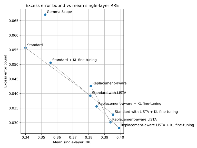
5 Discussion
In this post, I’ve presented several methods for improving the end-to-end performance of SAE replacement models. More so than any specific innovation, I want the take-away from this to be that more robust sparse representations are not only possible, but relatively unexplored. The LISTA encoder and replacement-aware training were literally the first things I tried once I became convinced of the inadequacy of the error node approach. Single-layer reconstruction error is simply not the correct optimization target if we want to explain how feature interactions determine model behavior. Taking a holistic view of the entire replacement model is an angle I expect to continue to be fruitful. In particular, I think directly tackling the problem of compounding reconstruction error (Section 4.3), as I have attempted to do here, is a neglected and important area of future research.
The main technical drawbacks of replacement-aware training are modestly increased computational and memory costs, forced sequential ordering of training runs, and the fact that it is not compatible with activation shuffling.15 The sequential ordering may not be too much of a burden in practice, since I found that warm-starting the layer \(i\) SAE from the layer \(i+1\) weights results in a moderate boost in performance for a given token budget (Appendix B.1), which could potentially be instead exchanged for shorter training runs on the earlier layers.
Replacement-aware training could be thought of as a variant of end-to-end training (Braun et al. 2024) adapted to the full replacement model. I previously found that end-to-end trained SAE replacement models outperform standardly trained ones on TinyStories. Even so, the much less computationally expensive next-layer replacement-aware SAEs outperformed those. I would guess that downstream reconstruction error and feature-space distortion are both capturing a similar signal—something like “sufficiency for the downstream layer to do its job”—but that the latter is more precisely targeted to our actual replacement model. I suspect that the explicit dependence on previously trained downstream SAEs is not strictly necessary. There might be something clever you can do based only on the statistics of the base model’s next layer activations, for example with something like information dropout (Achille and Soatto 2018).
Applying LISTA as the SAE encoder is a similar move to other recent works that have explored encoder variants, such as Matryoshka SAEs (Bussmann et al. 2025) and matching pursuit SAEs (Costa et al. 2025). While LISTA has been combined with Variational Auto-encoders (VAEs) in vision (Xiao et al. 2023), to my knowledge I’m the first to try it in this setting. Interestingly, I did not find improved performance of LISTA SAEs according to standard metrics (Section 4.6); their benefit appears to be realized only in the context of the full replacement model. It might be worth re-analyzing previous mediocre or negative results for variant SAEs (Baker and Li (2025) comes to mind; their framing, not mine!) through this lens. Another obvious angle for follow-up work would be to try out different numbers of iterations and sparsity schedules. I explored several variants of LISTA that didn’t make it into this post due to their lack of training stability.16 I think my implementation has a lot of room for improvement, particularly around finding a good parameter regularization scheme to ensure feature activation levels stay in a sane range.
Finally, encoder tuning (Section 3.2) may be worth investigating in its own right, possibly even as an alternative to replacement-aware training. It would definitely have to be refined somehow; I found that performance actually started decreasing with longer training runs, possibly resulting from the influence of the outliers mentioned in Section 4.2.17 A more stable version could potentially be used as an inexpensive way to generate more robust features out of off-the-shelf SAEs.
6 References
Achille, Alessandro, and Stefano Soatto. 2018. “Information Dropout: Learning optimal representations through noisy computation.” IEEE Transactions on Pattern Analysis and Machine Intelligence 40 (12): 2897–905.
Ameisen, Emmanuel, Jack Lindsey, Adam Pearce, et al. 2025. Circuit tracing: Revealing computational graphs in language models. https://transformer-circuits.pub/2025/attribution-graphs/methods.html.
Baker, Zachary, and Yuxiao Li. 2025. “Analysis of Variational Sparse Autoencoders.” arXiv [Cs.LG], September.
Bloom, Joseph, Curt Tigges, Anthony Duong, and David Chanin. 2024. SAELens. https://github.com/decoderesearch/SAELens.
Borgerding, Mark, and Philip Schniter. 2016. “Onsager-corrected deep learning for sparse linear inverse problems.” arXiv [Cs.IT], July.
Braun, Dan, Jordan Taylor, Nicholas Goldowsky-Dill, and Lee Sharkey. 2024. “Identifying functionally important features with end-to-end sparse dictionary learning.” arXiv [Cs.LG], May.
Bussmann, Bart, Patrick Leask, and Neel Nanda. 2024. “BatchTopK Sparse Autoencoders.” arXiv [Cs.LG], December.
Bussmann, Bart, Noa Nabeshima, Adam Karvonen, and Neel Nanda. 2025. “Learning multi-level features with Matryoshka sparse autoencoders.” arXiv [Cs.LG], March.
Caples, Diego, Jatin Nainani, Collum McDougall, and Rob Neuhaus. 2025. Scaling sparse feature circuit finding to Gemma 9B. https://www.lesswrong.com/posts/PkeB4TLxgaNnSmddg/scaling-sparse-feature-circuit-finding-to-gemma-9b.
Chen, Xiaohan, Jialin Liu, Zhangyang Wang, and Wotao Yin. 2018. “Theoretical linear convergence of unfolded ISTA and its practical weights and thresholds.” arXiv [Cs.LG], August.
Clark, Peter, Isaac Cowhey, Oren Etzioni, et al. 2018. “Think you have Solved Question Answering? Try ARC, the AI2 Reasoning Challenge.” arXiv [Cs.AI], March.
Costa, Valérie, Thomas Fel, Ekdeep Singh Lubana, Bahareh Tolooshams, and Demba Ba. 2025. “From flat to hierarchical: Extracting sparse representations with matching pursuit.” arXiv [Cs.LG], June.
Cunningham, Hoagy, Aidan Ewart, Logan Riggs, Robert Huben, and Lee Sharkey. 2023. “Sparse autoencoders find highly interpretable features in language models.” arXiv [Cs.LG], September.
Daubechies, I, M Defrise, and C De Mol. 2004. “An iterative thresholding algorithm for linear inverse problems with a sparsity constraint.” Communications on Pure and Applied Mathematics 57 (11): 1413–57.
Elhage, Nelson, Tristan Hume, Catherine Olsson, et al. 2022. Toy Models of Superposition. https://transformer-circuits.pub/2022/toy_model/index.html.
Gao, Hong-Ye, and Andrew G Bruce. 1997. “Waveshrink with firm shrinkage.” Statistica Sinica, 855–74.
Gao, Leo, Stella Biderman, Sid Black, et al. 2020. “The Pile: An 800GB dataset of diverse text for language modeling.” arXiv [Cs.CL], December.
Ge, Xuyang, Fukang Zhu, Wentao Shu, Junxuan Wang, Zhengfu He, and Xipeng Qiu. 2024. “Automatically identifying local and global circuits with linear computation graphs.” arXiv [Cs.LG], May.
Gemma Team, Morgane Riviere, Shreya Pathak, et al. 2024. “Gemma 2: Improving open language models at a practical size.” arXiv [Cs.CL], July.
Gorton, Liv. 2024. “The missing curve detectors of InceptionV1: Applying sparse autoencoders to InceptionV1 early vision.” arXiv [Cs.LG], June.
Gregor, Karol, and Yann LeCun. 2010. “Learning fast approximations of sparse coding.” International Conference on Machine Learning, June, 399–406.
Hanna, Michael, Mateusz Piotrowski, Jack Lindsey, and Emmanuel Ameisen. 2025. “Circuit-tracer: A new library for finding feature circuits.” Proceedings of the 8th BlackboxNLP Workshop: Analyzing and Interpreting Neural Networks for NLP (Stroudsburg, PA, USA), November, 239–49.
Heindrich, Lovis, Philip Torr, Fazl Barez, and Veronika Thost. 2025. “Do sparse autoencoders generalize? A case study of answerability.” arXiv [Cs.LG], February.
Hendrycks, Dan, Collin Burns, Steven Basart, et al. 2020. “Measuring massive multitask language understanding.” arXiv [Cs.CY], September.
Karvonen, Adam. 2025. “Revisiting end-to-end sparse autoencoder training: A short finetune is all you need.” arXiv [Cs.LG], March.
Kissane, Connor, Neel Nanda, and Arthur Conmy. 2024. “SAEs are highly dataset dependent: a case study on the refusal direction.” AI Alignment Forum, June.
Lieberum, Tom, Senthooran Rajamanoharan, Arthur Conmy, et al. 2024. “Gemma Scope: Open sparse autoencoders everywhere all at once on Gemma 2.” arXiv [Cs.LG], August.
Lindsey, Jack, Adly Templeton, Marcus Jonathan, Thomas Conerly, Joshua Batson, and Christopher Olah. 2024. Sparse crosscoders for cross-layer features and model diffing. https://transformer-circuits.pub/2024/crosscoders/index.html.
Liu, Jialin, Xiahan Chen, Zhangyang Wang, and Wotao Yin. 2019. “ALISTA: Analytic Weights Are As Good As Learned Weights in LISTA.”
Mallat, S G, and Zhifeng Zhang. 1993. “Matching pursuits with time-frequency dictionaries.” IEEE Transactions on Signal Processing 41 (12): 3397–415.
Marks, Samuel, Can Rager, Eric J Michaud, Yonatan Belinkov, David Bau, and Aaron Mueller. 2024. “Sparse feature circuits: Discovering and editing interpretable causal graphs in language models.” arXiv [Cs.LG], March.
Rajamanoharan, Senthooran, Tom Lieberum, Nicolas Sonnerat, et al. 2024. “Jumping ahead: Improving reconstruction fidelity with JumpReLU sparse autoencoders.” arXiv [Cs.LG], July.
Talmor, Alon, Jonathan Herzig, Nicholas Lourie, and Jonathan Berant. 2018. “CommonsenseQA: A question answering challenge targeting commonsense knowledge.” arXiv [Cs.CL], November.
Xiao, Pan, Peijie Qiu, Sungmin Ha, Abdalla Bani, Shuang Zhou, and Aristeidis Sotiras. 2023. “SC-VAE: Sparse Coding-based Variational Autoencoder with Learned ISTA.” arXiv [Cs.CV], March.
Yang, Jingcheng, Tianhu Xiong, Shengyi Qian, Klara Nahrstedt, and Mingyuan Wu. 2026. “Circuit tracing in vision-language models: Understanding the internal mechanisms of multimodal thinking.” arXiv [Cs.CV], February.
Zheng, Chujie, Hao Zhou, Fandong Meng, Jie Zhou, and Minlie Huang. 2023. “Large language models are not robust multiple choice selectors.” arXiv [Cs.CL], September.
7 Acknowledgements
I’d like to thank Curt Tigges for his mentorship during SPAR and for practical advice on proving out an early version of the LISTA-inspired encoder, and Billy Martin for helpful conversations and providing some of the GPU time used in these experiments.
Footnotes
Each CLT writes directly to every CLT following it. For any intermediate layer between \(i\) and \(m-1\), it must appear in exactly half of paths from \(i\) to \(m-1\), so it contributes 1/2 to the average path length. There are \(m-2-i\) intermediate layers, and an additional edge to \(m-1\) must be included in every path, so the average path length is \(\frac{m-2-i}{2} + 1=\frac{m-i}{2}\).↩︎
Note that I have deliberately omitted a sparsity-promoting regularization term on the SAE features, as in this post I will be exclusively using SAE architectures that achieve sparsity by other means.↩︎
The use of the KL term is admittedly questionable under this logic, at least for layers other than the final one! Its inclusion is purely pragmatic, as I did find it necessary in order to achieve the level of performance I was aiming for. I hope future work can find a more principled alternative. I report results both with and without the use of this term.↩︎
I did attempt a version of this that tuned all encoders in parallel, but I got much better results training them serially as written.↩︎
My best guess is that this is largely driven by adjusting the BatchTopK/JumpReLU thresholds to match the new statistics of the replacement model, as tuning those parameters in isolation also helps quite a bit, but I still saw additional gains when tuning the full set of encoder parameters.↩︎
This simplified the code and gave me marginally better performance on the hardware I was using.↩︎
I use an exponential moving average of the adaptive threshold in Equation 12, following the implementation in SAELens (Bloom et al. 2024).↩︎
The original paper used the soft shrinkage function \(h^{ss}_i(x) = \mathrm{sgn}(x)\cdot \max(|x|-\theta_i, 0)\), with threshold parameters \(\theta_i\) learned along with the update matrices and shared across iterations.↩︎
i.e., they are constrained to be non-negative and vary by many orders of magnitude. I also previously found them to be approximately log-normally distributed.↩︎
All reported results on CQA are over the validation split, so this won’t contaminate them.↩︎
I use this measure rather than the more common MSE because MSE varies by orders of magnitude across layers. The normalization factor makes these values directly comparable.↩︎
The sudden jump for the final layer is likely due to using the KL term of Equation 7 for the entire training run, rather than just for the last 20% of tokens, so there is potentially some trade-off happening there that isn’t present on the earlier layers.↩︎
“ish”, because the implicit objective here, the mean replacement model RRE, is actually one dimensional.↩︎
Gemma Scope uses JumpReLU, but we can adapt it in exactly the same way by adding a global offset to the individual feature thresholds, which is also what I did during the encoder tuning phase for those SAEs.↩︎
The replacement-aware loss function depends on having a complete example in context, since we have to run the next transformer layer on the SAE output.↩︎
For example, I attempted a run with a 10-iteration encoder, only to have the activations vanish in the replacement model even after encoder tuning. Due to the expense of this kind of training (each LISTA iteration uses the same compute as a vanilla encoder!), I gave up on trying to debug this.↩︎
I tried gradient clipping, using trimmed MSE as the loss function, and even outright dropping tokens generating extreme feature values, but none of these were successful.↩︎
I focus here on the cross-layer dynamics because that feels most natural for the residual stream SAEs discussed in the post, but it should be possible to extend this to be explicitly across token positions by adding nodes for attention-level features.↩︎
Citation
BibTeX citation:
@online{lloyd2026-scaling-replacement-aware-training,
  author = {Lloyd, Evan},
  title = {You don't need error nodes, you need better features},
  date = {2026-07-27},
  url = {https://elloworld.net/posts/you-dont-need-error-nodes-you-need-better-features/},
  langid = {en}
}
For attribution, please cite this work as:
Lloyd, Evan. 2026. You don't need error nodes, you need better features. July 27. https://elloworld.net/posts/you-dont-need-error-nodes-you-need-better-features/.
Appendix A: Implementation details
A.1 Training setup
I implemented the SAEs and SAE training pipeline used in this post without dependence on existing SAE libraries. I use SAELens (Bloom et al. 2024) only to load the weights for GemmaScope, which is then converted into my module format for evaluation consistent with the rest of my analysis. All source code is available on GitHub. The base model, Gemma-2-2B, is run using the huggingface transformers library. To implement replacement models, my code wraps a bare transformers model by replacing each transformer block with a module that first calls the original block, then replaces its output with the output of an attached SAE. For better performance, I include logic that stops the transformer computation as early as possible to obtain the needed activations.
The training pipeline uses the huggingface datasets library to fetch training data. All SAEs were trained using 50-100 million tokens from the pile-uncopyrighted(Gao et al. 2020) training split, as indicated in Table 3. KL fine-tuning and encoder tuning also use this dataset. All metrics presented in this post were run on 1 million tokens from the validation split of the same dataset. For efficiency, a consistent context length of 1024 tokens (as used in Gemma Scope) was used. Longer examples were truncated to that length, while smaller examples were concatenated greedily to attempt to fill each batch with as few padding tokens as possible. This was accomplished by looking ahead by up to 256 examples to fill in any gaps on a best-effort basis. Appropriate attention masks were set to account for multiple examples per batch row. Additionally, for each example I define a token mask to filter out padding and any other special tokens; my SAEs pass through the underlying transformer block’s output for these positions, and they are skipped when calculating loss and validation metrics.
All optimization is done using the PyTorch implementation of the Adam optimizer without weight decay. Following Gemma Scope (Lieberum et al. 2024), I use beta=[0, 0.999]. I found (by informal testing) that a learning rate of 1e-4 was effective, though I performed no formal sweep. BatchTopK thresholds were learned independently of the main optimizer using an exponential moving average with learning rate 1e-2. Following Karvonen (2025), I adaptively set the relative weights of each term in the loss functions such that they would have the same magnitude on a per-batch basis. I used a batch size of 2 complete context windows, for a total of 2048 tokens. When computing KL divergence loss terms, I aggregate using geometric mean rather than arithmetic mean, as I found this performed better in my earlier experiments with TinyStories.
All SAEs used a width of 16384 (approximately 7x the hidden dimension of 2304) to match with Gemma Scope. SAEs used either the BatchTopK (Equation 12) or LISTA (Equation 15) encoders, with sparsity parameters \(k_j\) set such that the final encoder output would have 100 expected non-zero entries. For BatchTopK this is simply \(k=100\); for LISTA, which I exclusively ran with 5 iterations, I used an increasing schedule after each iteration of [20, 40, 60, 80, 100].
For LISTA SAEs, I constrain the columns of the decoder to have unit norms by dividing them by their magnitudes after each training step. Additionally, the encoder weights are parametrized via PyTorch’s spectral_norm, and the per-iteration scalar values are soft-capped to 1 with tanh.
For memory and compute efficiency, the base model weights were cast to bfloat16, and PyTorch’s autocast feature is used wherever possible. SAE weights were trained in float32, but cast to bfloat16 once they were no longer needed in the replacement model used during training. Checkpoints are of course saved in full precision. All validations and benchmarks were done using the lower-precision weights and autocasting.
Encoder tuning (Section 3.2) was done over 1 million tokens from the same training set used in base training. The decoder weights are frozen for the entirety of this step. I found it most effective to apply Equation 11 to pairs of layers; the encoders for both SAE \(i\) and \(i+1\) are included in the optimizer parameters. To mitigate the outlier token problem (Section 4.2) and improve training stability, I apply a tanh softcap to the replacement model features of 10 times the maximum feature magnitude of the target baseline features.
A.2 Benchmark setup
To run the benchmarks reported in this post, I used the linked huggingface datasets MMLU (Hendrycks et al. 2020), CommonsenseQA (CQA) (Talmor et al. 2018), and the ARC Easy set (ARC-E) (Clark et al. 2018). For all benchmarks I use the n-shot template (line breaks added for clarity; exact spacing is as indicated with newline characters \n)
Question: {question}\n\n
A. {option[0]}\n
B. {option[1]}\n
C. {option[2]}\n
D. {option[3]}\n
E. {option[4]}\n
Answer: {answer_label}\n\n
Question: ...
Following the n-shot prefix, for the question being evaluated, the same template is filled in right until the colon after “Answer”, and the top logit for the predicted next token is taken as the model’s response.
For the “Valid answer” metric reported in various plots, I use the total proportion of times that the top-logit response corresponded to a valid option. Note that MMLU and ARC-E have only 4 valid options; option “E” is omitted from the n-shot template as well.
To implement PriDe (Zheng et al. 2023) (used only where specified), for each benchmark I take the first 5% of questions (including the n-shot prefix) as a debiasing sample. For each question in the sample, I copy the example with permuted options corresponding to every cyclic permutation (i.e. A, B, C, D -> B, C, D, A -> C, D, A, B -> D, A, B, C), which guarantees that every option appears once with each label. I then compute the mean probability (conditional on valid answer) assigned to each label over this sample as the prior probability for that label. Where I report “debiased” answers, these are the highest-probability valid option after dividing each label’s probability (again, conditioned on valid answer) by the corresponding prior. All of these probability calculations are performed in log-space (with, e.g. logsumexp operations) for better numerical precision.
Benchmark-specific details are highlighted below.
MMLU
For each MMLU subsection I use the corresponding “dev” split to generate a 5-shot prefix for each question. I evaluate over all examples from the “test” split of every subsection, excluding ones that exceed the maximum context length. This excludes the high_school_european_history, high_school_us_history, high_school_world_history, professional_law, and security_studies subsections. The resulting filtered set includes 11422 questions from 52 subsections.
CQA
CQA benchmark results are reported over the “validation” split. I use the first 10 examples to generate the 10-shot prompt, resulting in a total of 1211 questions. Note that I use the “train” split when performing CQA fine-tuning (Appendix A.3) so that results are not contaminated when evaluating CQA-finetuned replacement models.
ARC-E
I use the “test” split of the “Arc-Easy” subset of ARC. As in CQA, I take the first 10 examples to generate the 10-shot prompt. This dataset includes a small number of questions with a variable number of options, so to simplify analysis I discard all questions that do not have exactly 4 options. This leaves a total of 2355 questions.
A.3 CQA fine-tuning
For results that are marked as “CQA fine-tuned,” I repeat the appropriate version of KL fine-tuning (Section 3.1.1) with the standard SAE training dataset interleaved with questions and answers from the CQA “train” split in a 90%-10% mixture. Each CQA sample is formatted exactly as an n-shot prefix would be (Appendix A.2), with n drawn uniformly from the range (5, 25), the idea being that I didn’t want the question-answering-specific features to be overfit to specific token positions. The CQA dataset is allowed to repeat to guarantee that enough tokens can be drawn from it to reach the target fraction.
A.4 Gemma Scope encoder tuning
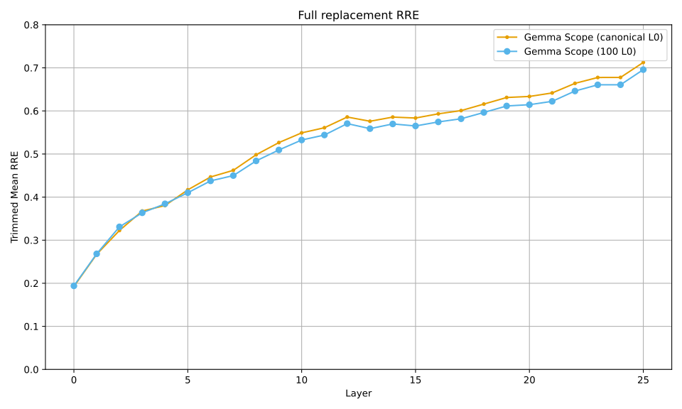
The Gemma Scope SAEs are implemented with the JumpReLU activation function, which is very similar to the inference-time BatchTopK except that the threshold varies for each feature. To adapt these SAEs into my framework, I add an additional parameter representing a global offset to the activation threshold, while keeping the base thresholds fixed. This avoids the need to set up the notoriously finicky kernel density estimation needed to tune the full set of thresholds. I learn this threshold offset in exactly the same way as I do for the BatchTopK SAEs, by exponential moving average. As can be seen in Figure 21, this is successful in adapting these SAEs to the desired sparsity of k=100. To make sure that this was as fair a comparison as possible, I also checked that tuning these SAEs to their “canonical” \(L_0\) values (which varied by layer, but were generally slightly less than 100), to which they were plausibly better adapted, did not improve performance. Indeed, the SAEs perform slightly better when tuned to \(L_0\)=100 at all layers:
Appendix B: Miscellaneous analyses
B.1 Warm-starting from the next layer SAE modestly boosts performance
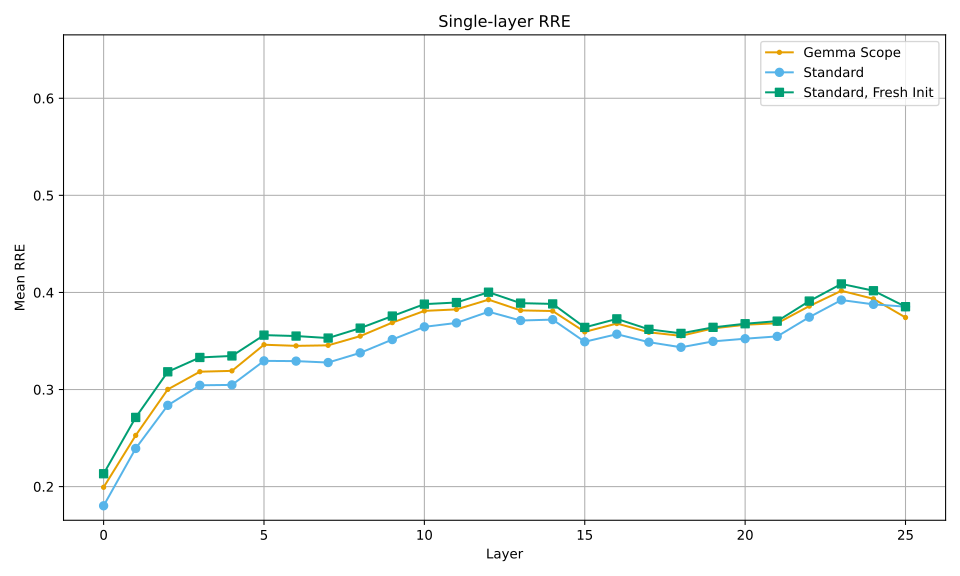
Replacement-aware training imposes a serial ordering on SAE training, since it requires that later layers already have their weights fixed. Given this, I thought it natural to warm start each SAE with the weights from the next layer, since it seems likely that adjacent layers will use similar representations. This may also encourage SAEs to retain features that are useful in multiple layers, since they will no longer have to discover them from scratch. As, to my knowledge, this is a novel initialization strategy for SAE training, I thought it would be worth a very brief examination of how effective it is. Below, I plot the single-layer RRE for standard training with or without this warm start:
| Loading ITables v2.8.0 from the internet... (need help?) |
This reveals a modest improvement for warm-starting, with a mean difference in RRE of 0.0206, or a mean relative difference of about 6%; the gap increases towards the start of the model (15% for the first layer, only 3.5% for the penultimate). For context, we can see in the chart that Gemma Scope (constrained to equivalent sparsity, see Appendix A.4), which was trained with much more data (4e9 tokens) but from a different distribution, lies somewhere in between the two. This is of course too crude an analysis to conclude much, but it does suggest that the warm start is training SAEs with a greater “effective number of training tokens.” Thus, for a given compute budget, an optimal training schedule using this initialization scheme could allocate shorter training runs for earlier layers. This may not be terribly exciting in practice, since earlier layers are already cheaper to run due to early stopping.
B.2 5e7 tokens is probably enough
As a sanity check that the single longer training run isn’t unfairly skewing the results, as well as a cursory investigation into what the training dynamics of replacement-aware training might look like, I compare validation statistics from the full 1e8 token next_layer training run with those from its 5e7 token checkpoints. Note that due to the warm start initialization (Appendix B.1), this isn’t quite identical to what a true 5e7 token training run would look like; the layer \(i\) SAE was initialized from the layer \(i+1\) SAE at the 1e8 token checkpoint, so even the earlier checkpoints for each layer have effectively seen more tokens. Still, there are interesting differences between the two replacement models:
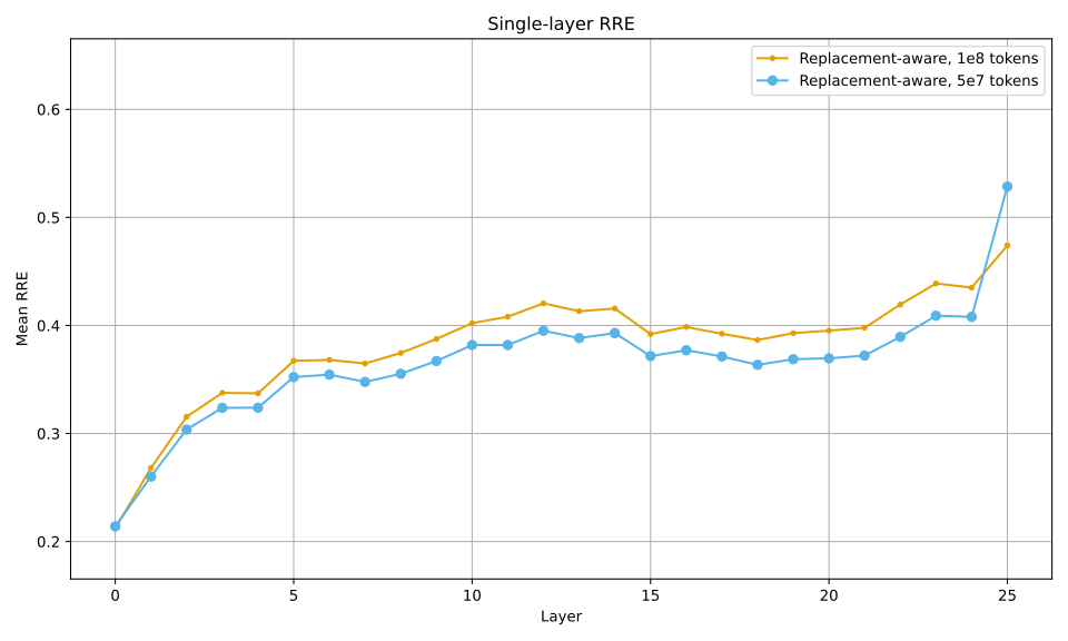
While the shorter run gets better RRE in the single-layer condition, the longer training run is marginally better in the full replacement condition, though only just:
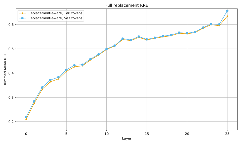
Repeating the analysis from Section 4.3 on these two replacement models seems to show that the longer training effectively increased the error-compounding-for-single-layer-accuracy trade-off:
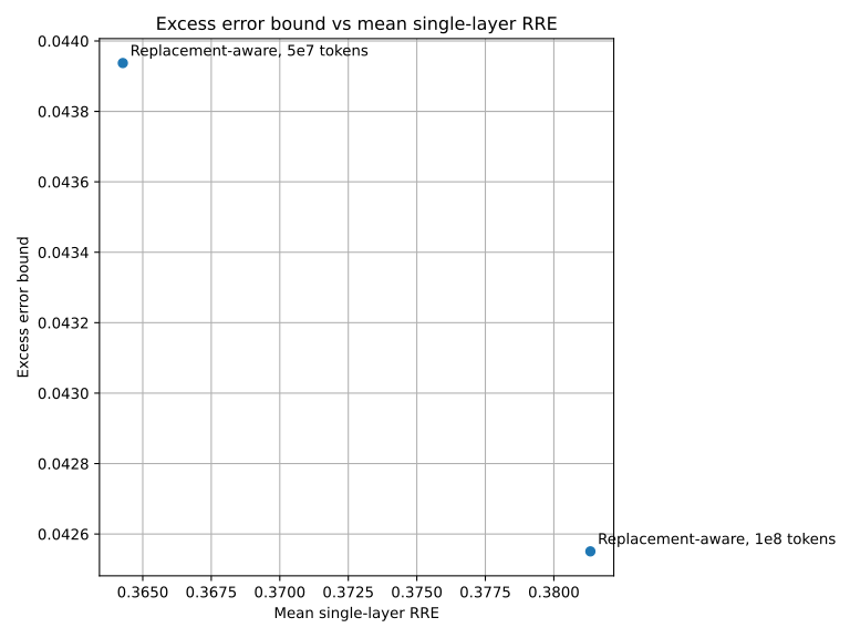
Yet, since the actual replacement model RRE barely improved, this could be an indication that the trade-off is sub-optimal; all else being equal, I think it’s reasonable to want the single-layer-replacement reconstruction to be as good as possible. It should be possible to tune this by changing the ratio of the current-layer and next-layer terms of Equation 7, which might be worth following up on.
Appendix C: Against error nodes; or, what’s the point of a feature circuit, anyway?
C.1 What’s the point of a feature circuit?
Aside from the concerns outlined in Section 2.2, I have a more fundamental issue with using error nodes in circuit discovery: the mechanisms this approach is capable of identifying are not expressible in terms of features alone, and that’s actually a major problem! This lack of representational sufficiency limits the validity of the circuit to the locality of a specific input. While this is fine when it comes to observational data, once we start trying to predict the results of feature-space interventions (e.g., steering), we are forced to step outside of this region of validity. The result is that any interventional predictions we try to make are subject to the same compounding error that the error nodes were meant to avoid. To explain, allow me to first sketch out my mental model of what we’re trying to accomplish with feature circuits in the first place.
If we take the superposition hypothesis (Elhage et al. 2022) seriously, then the activations we observe in a language model are in fact projections from a much higher dimensional space. Under this view, there is some unobserved “true” set of representations that evolve as computation progresses through the network18; the model has learned a compressed approximation of these representations. We can draw this schematically as
Note that since by hypothesis the \(F_i\) are higher dimensional than the activations \(\widehat{A}^{\emptyset}_i\), the operations represented by the downward arrows are not invertible; there are in general many possible configurations of features that could result in the observed activations. However, if we assume that the vector representations of the features are sparse, we can nevertheless infer them through the combination of sparse dictionary learning and sparse coding. This is the standard case for training SAEs as an interpretability tool.
I think that we should be more ambitious than merely identifying the features that are relevant to the model’s computation. In vision models, SAEs learn features corresponding to simple shapes like edges and textures in early layers, gradually converging on recognizable objects in the later layers (see, e.g., Gorton (2024)); there is a clear logic to this progression, and in principle it could be reverse-engineered into an interpretable algorithm. This should also be possible for language models! In my view, the point of a feature circuit is to use the inferred features to identify the feature-space mechanisms I have labeled \(C_i\). As I will now show, a full replacement model is a proxy on which we can validate arbitrary hypotheses about \(C_i\), including causal ones, but this property is destroyed by the addition of error nodes.
C.2 Replacement model as proxy
Recall the schematic depiction of the full replacement model from Figure 3. Because all of the labeled edges are deterministic, we can validly collapse some of them by incorporating the transformation into the node. In particular, we can use the fact that \(\widehat{F}_i^{[0..i]}=E_i(\widehat{A}^{[0..i-1]}_i)\) to remove the pre-encoded activation nodes. Furthermore, we can “lift” the right-pointing arrows to the feature level if we sacrifice causal equivalence at the activation level, using the fact that \(\widehat{F}_i^{[0..i]}=E_i\circ T_i\circ D_{i-1}(\widehat{F}_{i-1}^{[0..i-1]})\).
This model is obviously observationally equivalent to the replacement model on the remaining nodes, because all we have done is move some computations around without changing their values. It is not causally equivalent with respect to interventions on the activations since these are now leaf nodes, but it is causally equivalent with respect to interventions on the features. Since we are only interested in feature-level mechanisms, this is totally acceptable.
The point of these manipulations is of course that Figure 43 now matches the structure of Figure 42. The only difference is that the observed activations are now the replacement model activations \(\widehat{A}_i^{[0..m-1]}\) instead of the base model activations \(\widehat{A}^{\emptyset}_i\). Thus, this model is faithful to the original to the extent that these activations match.
To be clear, I am not claiming that the true mechanisms of the base model are literally “the composition of SAE encoder, transformer block, and SAE decoder,” which would be just as uninterpretable as when we started. What I am claiming is that this model is a proxy with which we can search for and validate simpler, actually interpretable functional relationships between the features. That is, by construction, when we make the intervention \(\mathbf{do}(\widehat{F}_i^{[0..m-1]}=f)\) in the replacement model, ablating the base model at layer \(i\) with the predicted activations \(\widehat{A}_i^{[0..m-1]}\) results in exactly the features at layer \(i+1\) as would be computed by the proxy, regardless of the original input \(x\).
C.3 Against error nodes
What happens when we add in error nodes that cancel out the SAE reconstruction error? We can employ similar manipulations as before to Figure 4 to get a graph supporting direct feature-to-feature interactions, though we still have an irreducible dependence on the base model activations:
The values of the error nodes are given by
\[ \delta_i=\widehat{A}_i^{\emptyset} - D_i \circ E_i(\widehat{A}_i^{\emptyset}), \tag{17}\]
i.e. the values that exactly cancel the SAE reconstruction error. The features are given by
\[ \widehat{F}^{\{i\}}_i=E_i \circ T_i(D_{i-1}(\widehat{F}^{\{i-1\}}_{i-1}) + \delta_{i-1}). \tag{18}\]
By construction, this model computes the single-layer-replacement features \(\widehat{F}^{\{i\}}_i\); it is a useful proxy for purely observational data. However, consider the causal intervention \(\mathbf{do}(\widehat{F}^{\{0\}}_0=f')\) when the original input is \(x\). To clean up the notation for the sake of this argument, let \(F_i\) refer to the “natural” (pre-intervention) values that the corresponding more ornamented nodes would take in the graph for this input, and let \(F_i'\) refer to their post-intervention values. Additionally, let \(A_i\) refer to the base model activations \(\widehat{A}^{\emptyset}_i\) for the input \(x\). Then we have
\[ \begin{align} \underline{\underline{F_1}}'&=E_1 \circ T_1(D_{0}(f') + \delta_{0})\\ &=E_1 \circ T_1(A_0 + D_0(f') - D_0(\underline{F_0})). \end{align} \]
Notably, the result is no longer equivalent to the encoder applied to the layer 1 base model activations; we have taken a step away from that activation in the direction defined by the difference between the counterfactual layer 0 features and the ones we actually observed on this input. And of course we have, because that’s what a causal intervention is! However, the important thing to note here is that the result now contains two sequential uses of SAE encoders; the outer \(E_1\), and the inner \(\underline{F_0}\), since \(\underline{F_0}=E_0(A_0)\). Note that I have underlined terms according to the number of sequential encoders they depend on. Proceeding to the next layer, we have
\[ \begin{align} \underline{\underline{\underline{F_2}}}' &= E_2\circ T_2(D_{1}(\underline{\underline{F_1}}') + \delta_{1})\\ &=E_2 \circ T_2(A_1 + D_1(\underline{\underline{F_1}}') - D_1(\underline{F_1})), \end{align} \]
which now depends on three sequential encodings: \(E_2\) applied to a value that depends on \(\underline{\underline{F_1}}'\), which itself depended on two sequential encodings. Obviously, this pattern continues for any remaining layers in the model; the final layer features depend on \(m-1\) sequential encodings, exactly as in the full replacement model.
I would like to emphasize that this dependence on serial reconstructions is not an accidental property of the way I have chosen to set up the causal graphs. The fundamental reason error nodes cannot help in this situation is that interventions on features must have downstream consequences or else be meaningless. And how else could we measure the downstream impact on a later layer’s features, than by applying that layer’s encoder? Thus, it seems to me that we are forced to contend with compounding reconstruction error; improving the accuracy of causal predictions depends on reducing it, not on some clever scheme to bypass it.